Every Little Thing Heat Does is Magic

Notes

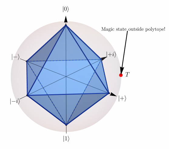
Thumbnail adapted from Geometric Analysis of the Stabilizer Polytope for Few-Qubit Systems.

These notes are based on Every Little Thing Heat Does Is Magic.

• Central question: is it possible to “measure” quantum magic without full state tomography? Yes!

  • The authors develop thermodynamic witnesses for quantum magic: energy and heat measurements.
  • We have the notion of an entanglement gap: energies which are inaccessible to separable states when we consider the Hamiltonian itself as a witness. It turns out that we can do something analogous for magic. See, for example: Entanglement observables and witnesses for interacting quantum spin systems and Multipartite entanglement in spin chains.
  • Much of the paper which we are currently discussing is also based on one of the previous works by the authors: Heat as a Witness of Quantum Properties (Phys. Rev. Lett. 134, 050401). There, they establish some of the central mathematical results here and show how heat can be used as, e.g., a witness of entanglement and for the certification of coherence.

As discussed in the introduction:

“We introduce the notion of the stabilizer gap, defined as the difference between the energy of the groundstate and the minimum energy achievable by any stabilizer state.”

Thus: system’s energy $<$ stabilizer threshold $\rightarrow$ non-stabilizer state.

Short Review on Stabilizer Resource Theory

See Nielsen & Chuang, page 454 (10th Edition):

“Suppose $S$ is a subgroup of the Pauli group, and define $V_S$ to be the set of $n$-qubit states which are fixed by every element of $S$. Then $V_S$ is the vector space stabilized by $S$, and $S$ is said to be the stabilizer of the space $V_S$.”

[!note

highlight-blue] Stabilizer code example

A simple example would be the single stabilizer state associated with the generators given by $\boldsymbol{S} = \langle X_1X_2, Z_1Z_2 \rangle$, which yields the stabilizer state $\ket{\psi} = \ket{00} + \ket{11}$ (we keep it unnormalized for simplicity).

Similarly, if $n=3$ and $\boldsymbol{S} = \langle X_1X_2 \rangle$, we have $\mathrm{rank}(\boldsymbol{S}) = 1$; thus, $\mathrm{dim} V_\mathrm{\boldsymbol{S}} = 2 ^{n - \mathrm{rank}(\boldsymbol{S})} = 4$. And, in fact, the associated subspace is:

\[V_\mathrm{\boldsymbol{S}} = \mathrm{span} \left\{ \lvert 000 \rangle,\quad \lvert 001 \rangle,\quad \lvert 110 \rangle,\quad \lvert 111 \rangle \right\}\]

A way to measure “non-stabilizerness” is given, for instance, in Geometric Analysis of the Stabilizer Polytope for Few-Qubit Systems, for the space of $n$ qudits (local dimension $d$):

There, $\lVert \dots \rVert_1$ is the trace distance. The problem with such measures, however, is the fact that one needs knowledge of the full density matrix – something which would require full state tomography.

Quantum Thermodynamics Framework

We consider a thermal Gibbs state, in equilibrium with the environment $E$ at inverse temperature $\beta$:

[!note

highlight-green] Thermal operations

We consider the class of thermal operations on the system (cf. Irreversible entropy production, from quantum to classical (PDF)) $\mathcal{E}$, which are CPTP:

\[\mathcal{E}(\rho_S) := \operatorname{tr}_E \!\left[\, U(\rho_S \otimes \gamma_E)U^\dagger \,\right].\]

These are operations such that:

\[[U, H_S \otimes \mathbb{1}_E + \mathbb{1}_S \otimes H_E] = 0\]

where $U$ is a global system-environment unitary. That is, these are operations where no energy is “trapped in the interaction”. This often makes the quantum thermodynamic description (e.g. first law) much simpler and less ambiguous.

The energy exchanges of the system and environment are:

respectively. We thus define the energy gained by $E$ as the heat, so that $Q(\rho_S) \equiv \Delta E_E$.

The problem with this approach, however, is the fact that only the diagonal terms (populations) are relevant to the thermodynamics of the process. The authors propose a more general description through a memory-based framework.

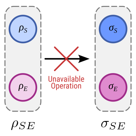
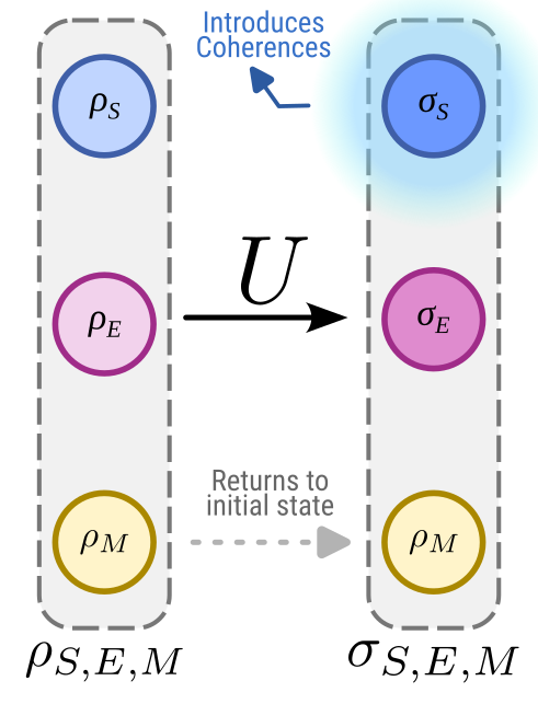
The idea is:

• We introduce a new ancillary system $M$.
• Initially, (i) it has no correlations with $S$ and $E$, but the unitary acts globally on all three constituents, while (ii) still obeying the conditions for a thermal operation.
• We also include a third constraint that (iii) requires that the memory subsystem returns to its initial state at the end of the evolution. That is: $\rho_M(\text{start}) = \rho_M(\text{end})$ (which implies that the memory neither absorbs nor gives energy to either of the other two constituents).
• Thus: the memory subsystem acts as an ancilla which allows for the conversion of coherences into population changes in $S$ and $E$.

[!note

highlight-green] Quantum catalysis

For a review on this topic, see Catalysis in Quantum Information Theory – Rev. Mod. Phys. 96, 025005 (2024).

The idea behind catalysis is to introduce additional degrees of freedom which enable certain transitions/operations which would not be possible otherwise (be it due to experimental limitations, conservation laws, or physical constraints).

Under such circumstances, we can then bound the minimum/maximum amount of heat exchanged with the environment through a semidefinite problem:

Naturally, this is a very hard optimization problem, given the enormous size of the search space. However, as some of the authors have done in Heat as a Witness of Quantum Properties (Phys. Rev. Lett. 134, 050401), it is then possible to convert this to a much simpler problem, where the heat is given in terms of effective inverse temperatures $\beta_{c/h}$:

These temperatures, in turn, are set by the condition $F[\gamma_S(\beta_{c/h})] = F(\rho_S)$, where the free energy is given by $F(\rho) := \mathrm{Tr}[\rho H_S] - \frac{1}{\beta}S(\rho)$. Similarly, the average energy is defined as $E(\rho) := \mathrm{Tr}[\rho H_S]$.

The question is now: what happens when the initial state $\rho_S$ is constrained to a subset of interest $\mathcal{S}$, such as, e.g., stabilizer or separable states? For a convex set, the minimum/maximum quantities above will establish a set-dependent bound, such that the heat exchange $Q$ will lie in the interval $Q \in [Q_c, Q_h] : \forall : \rho_S \in \mathcal{S}$. In this scenario, heat will function as a witness, and any observed value outside this range will certify that the underlying state $\rho_S$ also lies outside $\mathcal{S}$: in our particular example, heat will then act as a witness of non-stabilizerness. Note how this approach avoids full-state tomography! It is not necessary to have full knowledge of the state $\rho_S$.

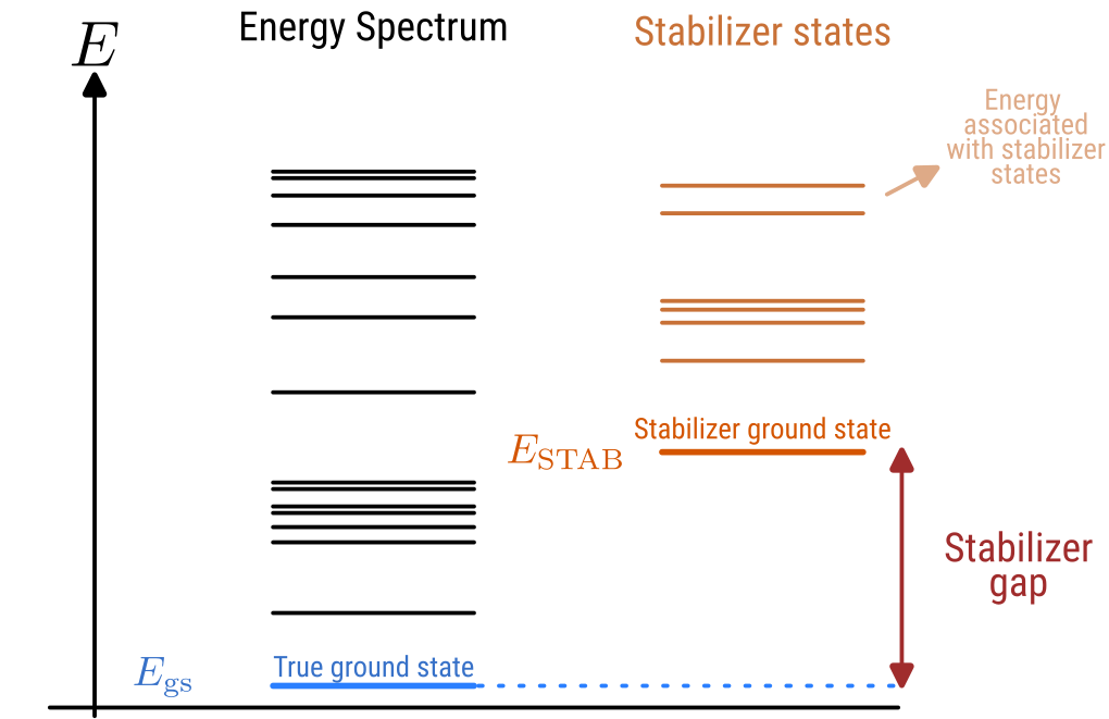
A relevant notion is the idea of stabilizer ground-state:

That is, among the stabilizer states within the stabilizer polytope, defined as the convex set constructed from all pure stabilizer states:

which of these states minimizes the energy, given the Hamiltonian $H_S$? Naturally, a quantum state is said to be a non-stabilizer state if it does not belong to this set.

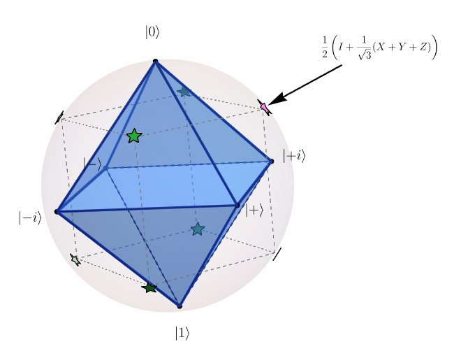
[!note

highlight-green] Stabilizer polytope in single-qubit case

In the case of qubits, there is a very nice geometrical picture: the stabilizer polytope is simply the octahedron whose vertices are given by the six eigenstates of the Pauli matrices $X, Y, Z$. Plotting this over the Bloch sphere, we get:

Thus, from the convexity of this set, any “non-extremal” stabilizer state will yield a higher energy than the stabilizer ground-state energy $E_{\mathrm{STAB}}(H_S)$. For instance, if $\rho_1$ and $\rho_2$ are stabilizer states, the energy associated with their convex mixture $\alpha \rho_1 + (1 - \alpha) \rho_2$ is

Assuming that $\rho_1$ is the stabilizer ground-state, we have $\operatorname{tr}(H_S \rho_2) \geqslant \operatorname{tr}(H_S \rho_1)$, and therefore $E_\mathrm{mixture} \geqslant E_{\mathrm{STAB}}(H_S)$.

However, what happens when we have a non-stabilizer state? For that, we introduce the witness:

By the convexity argument above, one generally has $\mathrm{Tr}[\sigma_{\mathrm{STAB}} W_H] > 0$ for any stabilizer state $\sigma_{\mathrm{STAB}}$. However, any state $\rho_S$ which yields a negative value for this witness:

is guaranteed to be non-stabilizer! This serves as a scaffold for another meaningful definition, namely, that of a stabilizer gap:

This essentially answers the question: how far away is the stabilizer ground-state energy from the true ground-state of the Hamiltonian?

[!note

highlight-blue] Single-qubit example

Let us consider normalized ($h_x^2 + h_y^2 + h_z^2 = 1$) Hamiltonians $H = h_x \sigma_X + h_y \sigma_y + h_z \sigma_z$. In this case, the stabilizer gap is:

\[\delta_{\mathrm{STAB}}(H) = 1 - \max_{i \in \{x,y,z\}} \lvert h_i\rvert.\]

This result has a nice geometrical intuition: the stabilizer gap is simply “the smallest distance” between the point where $H_S$ lies in the Bloch sphere and the extreme points of the polytope. As the authors argue, the maximum stabilizer gap $1 - 1/\sqrt{3}$ is achieved through:

\[H = -\frac{1}{\sqrt{3}}(\mathbf{f}\cdot\boldsymbol{\sigma}), \qquad \mathbf{f} = (f_x, f_y, f_z) \in\{\pm 1\}^3,\]

which has coordinates $-\frac{1}{\sqrt{3}}(f_x, f_y, f_z)$ in the Bloch sphere.

In fact, we can see that the point above defines eight points in the Bloch sphere. In particular, one of these states corresponds to the T-state:

\[\ket{T}\!\bra{T} = \frac{1}{2} \left[ I + \frac{1}{\sqrt{3}}(X+Y+Z) \right].\]

What about a less trivial example with two qubits?

[!note

highlight-blue] Two-qubit example

In the paper, they introduce a special class of stabilizer Hamiltonians:

\[H[S, \operatorname{gen}(S)] := - \sum_{g \in \operatorname{gen}(S)} g.\]

In this case, it is evident that the stabilizer gap is zero. With that in mind, they introduce an example where one has:

\[H_{\mathrm{Bell}}(\varepsilon) = H_{0, \mathrm{STAB}} + \varepsilon (Z \otimes I - I \otimes Z),\]

where

\[H_{0, \mathrm{STAB}} = - X \otimes X - Z \otimes Z = H_{\mathrm{Bell}}(\varepsilon = 0),\]

is a stabilizer Hamiltonian, with ground state $\Phi^{+} := (\ket{00} + \ket{11})/\sqrt{2}$ – which is clearly stabilized by the underlying generators/terms in $H_{0, \mathrm{STAB}}$. Note how the “perturbation” term in $H_{\mathrm{Bell}}(\varepsilon)$ does not commute with the stabilizer part/Hamiltonian above. The energies we get are:

\[E_{\mathrm{GS}}\!\left[H_{\Phi}(\varepsilon)\right] = \min\!\left\{-2,\; 1 - \sqrt{1 + 4\varepsilon^2}\right\},\] \[E_{\mathrm{STAB}}\!\left[H_{\Phi}(\varepsilon)\right] = \min\!\left\{-2,\; 1 - 2\varepsilon\right\}.\]

This can be seen by noting that $\langle \Phi^{+} \rvert H_{\mathrm{Bell}}(\varepsilon) \lvert \Phi^{+} \rangle = -2$ for $\varepsilon \in [0, \sqrt{2}]$. However, note that for the product state $\ket{01}$ we have $\langle 01 \rvert H_{\mathrm{Bell}}(\varepsilon) \lvert 01 \rangle = 1 - 2 \varepsilon$. This means that we have a transition at $\varepsilon = \sqrt{2}$ where the Bell state ceases to be the stabilizer ground-state, and a stabilizer gap emerges.

In the paper, they consider states of the type

\[\ket{\psi(\theta,\phi)} = I \otimes e^{-i\phi X/2} \left( \cos\theta\,\ket{00} + \sin\theta\,\ket{11} \right).\]

where the corresponding energy is

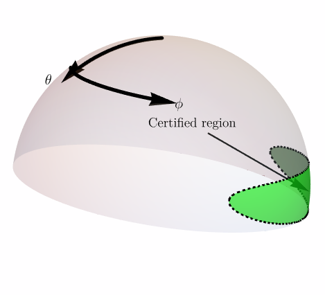
\[E(\theta,\phi,\varepsilon) = -\cos\phi\,\sin(2\theta) -\cos(2\theta) +\varepsilon\bigl(1-\cos(2\theta)\bigr).\]

We can now simply look for states which, following the parametrization above, obey $E(\theta,\phi,\varepsilon) < E_{\mathrm{STAB}}$. Such states whose energy is larger than the true ground-state energy, but smaller than the stabilizer ground-state energy, are guaranteed to have magic. We highlight such states, given by the pairs $(\phi, \theta)$, in the spherical plots below.

For instance, for $\varepsilon = 3/2$ we have:

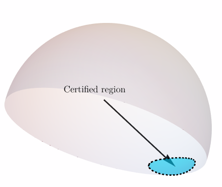
And for $\varepsilon = 3$:

Note how the certifiable region shrinks for larger $\varepsilon$.

Nevertheless, as the authors point out, this Hamiltonian is somewhat fine-tuned, and as long as we consider sufficiently generic “perturbations”, one usually has a non-vanishing stabilizer gap (cf. Eq. 35).

[!note

highlight-red] Some important caveats

The authors also bring attention to two important edge cases here:

• The first is, as we have seen above, the scenario where the stabilizer gap was zero: if the GS of the Hamiltonian is also a stabilizer state (or if its ground space contains one), the method is blind to non-stabilizer states and the stabilizer gap vanishes.
• However, not only that: as the authors point out in the example of the Heisenberg spin chain, which is not a stabilizer Hamiltonian, the Hamiltonian itself is not a stabilizer, although its ground state $\ket{0}^{\otimes n}$ is. In this case, the stabilizer gap is zero, despite the non-stabilizerness of the Hamiltonian itself.

For some related work, see:

• Operational Definition of the Temperature of a Quantum State (Phys. Rev. Lett. 130, 040401)